Interaction between phylogenetic uncertainty and sensitivity to species sampling - Phylogenetic Linear Regression
Source:R/tree_samp_phylm.R
tree_samp_phylm.RdPerforms analyses of sensitivity to species sampling by randomly removing species and detecting the effects on parameter estimates in a phylogenetic linear regression, while evaluating uncertainty in trees topology.
tree_samp_phylm(
  formula,
  data,
  phy,
  n.sim = 30,
  n.tree = 2,
  breaks = seq(0.1, 0.5, 0.1),
  model = "lambda",
  track = TRUE,
  ...
)
Arguments
| formula | The model formula |
|---|---|
| data | Data frame containing species traits with row names matching tips
in |
| phy | A phylogeny (class 'phylo') matching |
| n.sim | The number of times species are randomly deleted for each
|
| n.tree | Number of times to repeat the analysis with n different trees picked randomly in the multiPhylo file. |
| breaks | A vector containing the percentages of species to remove. |
| model | The phylogenetic model to use (see Details). Default is |
| track | Print a report tracking function progress (default = TRUE) |
| ... | Further arguments to be passed to |
Value
The function samp_phylm returns a list with the following
components:
formula: The formula
full.model.estimates: Coefficients, aic and the optimised
value of the phylogenetic parameter (e.g. lambda or kappa) for
the full model without deleted species.
sensi.estimates: A data frame with all simulation
estimates. Each row represents a model rerun with a given number of species
n.remov removed, representing n.percent of the full dataset.
Columns report the calculated regression intercept (intercept),
difference between simulation intercept and full model intercept (DIFintercept),
the percentage of change in intercept compared to the full model (intercept.perc)
and intercept p-value (pval.intercept). All these parameters are also reported
for the regression slope (DIFestimate etc.). Additionally, model aic value
(AIC) and the optimised value (optpar) of the phylogenetic
parameter (e.g. kappa or lambda, depending on the phylogenetic model
used) are reported. Lastly we reported the standardised difference in intercept
(sDIFintercept) and slope (sDIFestimate).
sign.analysis For each break (i.e. each percentage of species
removed) this reports the percentage of statistically significant (at p<0.05)
intercepts (perc.sign.intercept) over all repetitions as well as the
percentage of statisticaly significant (at p<0.05) slopes (perc.sign.estimate).
data: Original full dataset.
#' @note Please be aware that dropping species may reduce power to detect
significant slopes/intercepts and may partially be responsible for a potential
effect of species removal on p-values. Please also consult standardised differences
in the (summary) output.
Details
This function randomly removes a given percentage of species (controlled by
breaks) from the full phylogenetic linear regression, fits a phylogenetic
linear regression model without these species using phylolm,
repeats this many times (controlled by n.sim), stores the results and
calculates the effects on model parameters. It repeats this operation using n trees,
randomly picked in a multiPhylo file.
All phylogenetic models from phylolm can be used, i.e. BM,
OUfixedRoot, OUrandomRoot, lambda, kappa,
delta, EB and trend. See ?phylolm for details.
Currently, this function can only implement simple linear models (i.e. \(trait~ predictor\)). In the future we will implement more complex models.
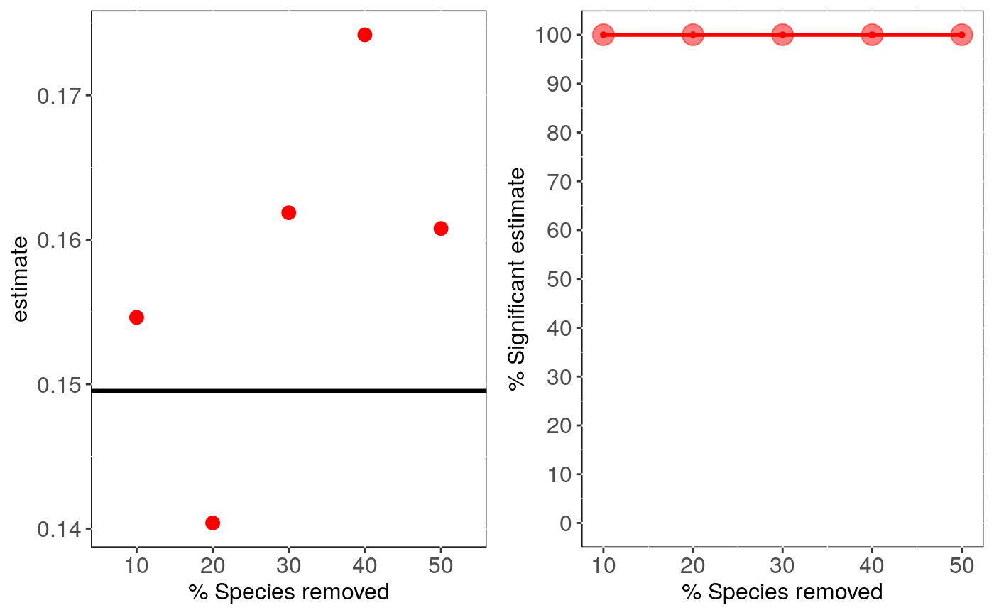
Output can be visualised using sensi_plot.
References
Paterno, G. B., Penone, C. Werner, G. D. A. sensiPhy: An r-package for sensitivity analysis in phylogenetic comparative methods. Methods in Ecology and Evolution 2018, 9(6):1461-1467
Werner, G.D.A., Cornwell, W.K., Sprent, J.I., Kattge, J. & Kiers, E.T. (2014). A single evolutionary innovation drives the deep evolution of symbiotic N2-fixation in angiosperms. Nature Communications, 5, 4087.
Ho, L. S. T. and Ane, C. 2014. "A linear-time algorithm for Gaussian and non-Gaussian trait evolution models". Systematic Biology 63(3):397-408.
See also
Examples
if (FALSE) { # Load data: data(alien) # Run analysis: samp <- tree_samp_phylm(log(gestaLen) ~ log(adultMass), phy = alien$phy, data = alien$data, n.tree = 5, n.sim=10) summary(samp) head(samp$sensi.estimates) # Visual diagnostics sensi_plot(samp) sensi_plot(samp, graphs = 1) sensi_plot(samp, graphs = 2) } # \dontshow{ # Load data: data(alien) # Run analysis: samp <- tree_samp_phylm(log(gestaLen) ~ log(adultMass), phy = alien$phy, data = alien$data, n.tree = 1, n.sim=1)#> Warning: NA's in response or predictor, rows with NA's were removed#> Warning: Some phylo tips do not match species in data (this can be due to NA removal) species were dropped from phylogeny or data#>#> | | | 0% | |======================================================================| 100%summary(samp)#>#> % Species Removed % Significant Intercepts Mean Intercept Change (%) #> 1 10 100 1.7 #> 2 20 100 3.3 #> 3 30 100 0.9 #> 4 40 100 2.5 #> 5 50 100 3.4 #> Mean sDIFintercept % Significant Estimates Mean Estimate Change (%) #> 1 -0.6002325 100 3.4 #> 2 1.1585638 100 6.1 #> 3 -0.3100876 100 8.2 #> 4 0.8701820 100 16.5 #> 5 -1.2022838 100 7.5 #> Mean sDIFestimate #> 1 0.4131880 #> 2 -0.7436704 #> 3 1.0016718 #> 4 2.0032507 #> 5 0.9136294#> Warning: `fun.y` is deprecated. Use `fun` instead.#> Warning: `fun.y` is deprecated. Use `fun` instead.#> Warning: `fun.y` is deprecated. Use `fun` instead.# }
