Interaction between phylogenetic uncertainty and influential clade detection - Phylogenetic Logistic Regression
Source:R/tree_clade_phyglm.R
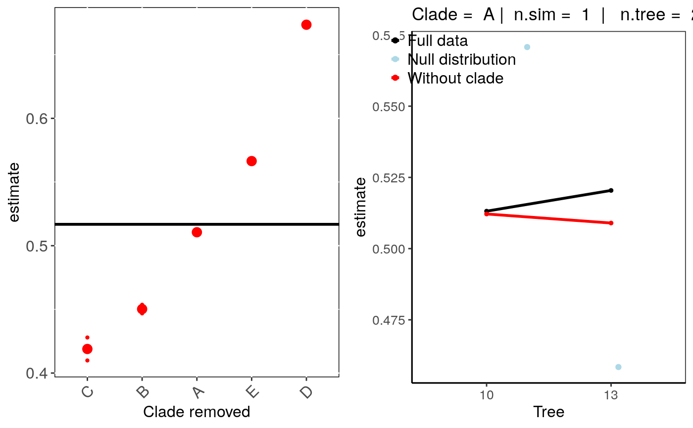
tree_clade_phyglm.RdEstimate the impact on model estimates of phylogenetic logistic regression after removing clades from the analysis and evaluating uncertainty in trees topology.
tree_clade_phyglm(
  formula,
  data,
  phy,
  clade.col,
  n.species = 5,
  n.sim = 100,
  n.tree = 2,
  btol = 50,
  track = TRUE,
  ...
)
Arguments
| formula | The model formula |
|---|---|
| data | Data frame containing species traits with row names matching tips
in |
| phy | A phylogeny (class 'multiPhylo', see ? |
| clade.col | The column in the provided data frame which specifies the clades (a character vector with clade names). |
| n.species | Minimum number of species in a clade for the clade to be
included in the leave-one-out deletion analysis. Default is |
| n.sim | Number of simulations for the randomization test. |
| n.tree | Number of times to repeat the analysis with n different trees picked
randomly in the multiPhylo file.
If NULL, |
| btol | Bound on searching space. For details see |
| track | Print a report tracking function progress (default = TRUE) |
| ... | Further arguments to be passed to |
Value
The function clade_phyglm returns a list with the following
components:
formula: The formula
full.model.estimates: Coefficients, aic and the optimised
value of the phylogenetic parameter (e.g. lambda) for the full model
without deleted species.
sensi.estimates: A data frame with all simulation
estimates. Each row represents a deleted clade for a tree iteration. Columns report the calculated
regression intercept (intercept), difference between simulation
intercept and full model intercept (DIFintercept), the percentage of change
in intercept compared to the full model (intercept.perc) and intercept
p-value (pval.intercept). All these parameters are also reported for the regression
slope (DIFestimate etc.). Additionally, model aic value (AIC) and
the optimised value (optpar) of the phylogenetic parameter
(e.g. kappa or lambda, depending on the phylogenetic model used)
are reported.
null.dist: A data frame with estimates for the null distributions
for all clades analysed.
data: Original full dataset.
errors: Clades and/or trees where deletion resulted in errors.
Details
Currently only logistic regression using the "logistic_MPLE"-method from
phyloglm is implemented.
This function sequentially removes one clade at a time, fits a phylogenetic
logistic regression model using phyloglm and stores the
results. The impact of of a specific clade on model estimates is calculated by the
comparison between the full model (with all species) and the model without
the species belonging to a clade. It repeats this operation using n trees,
randomly picked in a multiPhylo file.
Additionally, to account for the influence of the number of species on each clade (clade sample size), this function also estimates a null distribution of slopes expected for the number of species in a given clade. This is done by fitting models without the same number of species in the given clade. The number of simulations to be performed is set by 'n.sim'. To test if the clade influence differs from the null expectation for a clade of that size, a randomization test can be performed using 'summary(x)'.
clade_phyglm detects influential clades based on
difference in intercept and/or slope when removing a given clade compared
to the full model including all species. This is done for n trees in the multiphylo file.
Currently, this function can only implements simple logistic models (i.e. \(trait~ predictor\)). In the future we will implement more complex models.
Output can be visualised using sensi_plot.
References
Paterno, G. B., Penone, C. Werner, G. D. A. sensiPhy: An r-package for sensitivity analysis in phylogenetic comparative methods. Methods in Ecology and Evolution 2018, 9(6):1461-1467
Ho, L. S. T. and Ane, C. 2014. "A linear-time algorithm for Gaussian and non-Gaussian trait evolution models". Systematic Biology 63(3):397-408.
See also
Examples
if (FALSE) { # Simulate Data: set.seed(6987) mphy = rmtree(150, N = 30) x = rTrait(n=1,phy=mphy[[1]]) X = cbind(rep(1,150),x) y = rbinTrait(n=1,phy=mphy[[1]], beta=c(-1,0.5), alpha=.7 ,X=X) cla <- rep(c("A","B","C","D","E"), each = 30) dat = data.frame(y, x, cla) # Run sensitivity analysis: tree_clade <- tree_clade_phyglm(y ~ x, phy = mphy, data = dat, n.tree = 10, n.sim = 10, clade.col = "cla") # To check summary results and most influential clades: summary(tree_clade) # Visual diagnostics for clade removal: sensi_plot(tree_clade) # Specify which clade removal to plot: sensi_plot(tree_clade, "B") sensi_plot(tree_clade, "C", graphs = 2) sensi_plot(tree_clade, "D", graphs = 2) } # \dontshow{ set.seed(6987) mphy = rmtree(150, N = 30) x = rTrait(n=1,phy=mphy[[1]]) X = cbind(rep(1,150),x) y = rbinTrait(n=1,phy=mphy[[1]], beta=c(-1,0.5), alpha=.7 ,X=X) cla <- rep(c("A","B","C","D","E"), each = 30) dat = data.frame(y, x, cla) # Run sensitivity analysis: tree_clade <- tree_clade_phyglm(y ~ x, phy = mphy, data = dat, n.tree = 2, n.sim = 1, clade.col = "cla")#>#> | | | 0% | |=================================== | 50% | |======================================================================| 100%#> $Estimate #> clade.removed N.species estimate DIFestimate Change (%) Pval #> 4 D 30 0.6734920 0.156708757 30.35 1.144792e-06 #> 3 C 30 0.4189061 -0.097877230 18.90 7.741017e-05 #> 2 B 30 0.4502398 -0.066543453 12.85 1.328916e-05 #> 5 E 30 0.5664308 0.049647543 9.65 4.854874e-06 #> 1 A 30 0.5105626 -0.006220664 1.20 1.591829e-05 #> m.null.estimate Pval.randomization Significant (%) #> 4 0.5366828 0.0 100 #> 3 0.4845104 0.0 100 #> 2 0.5469125 0.0 100 #> 5 0.5024571 0.5 50 #> 1 0.5319009 0.5 50 #> #> $Intercept #> clade.removed N.species intercept DIFintercept Change (%) Pval #> 4 D 30 -0.9033605 -0.13145386 17.05 1.144792e-06 #> 3 C 30 -0.7937692 -0.02186248 5.20 7.741017e-05 #> 2 B 30 -0.4858454 0.28606132 37.00 1.328916e-05 #> 5 E 30 -0.9960052 -0.22409851 29.05 4.854874e-06 #> 1 A 30 -0.7242611 0.04764556 6.15 1.591829e-05 #> m.null.intercept Pval.randomization Significant (%) #> 4 -0.7520597 0.0 100 #> 3 -0.6963086 0.0 100 #> 2 -0.8444144 0.0 100 #> 5 -0.7636749 0.5 50 #> 1 -0.7652482 0.5 50 #>#> Warning: Clade argument was not defined. Plotting results for clade: A #> Use clade = 'clade name' to plot results for other clades#> Warning: `fun.y` is deprecated. Use `fun` instead.# }
