Intraspecific variability - Phylogenetic Logistic Regression
Source:R/intra_phyglm.R
intra_phyglm.RdPerforms Phylogenetic logistic regression evaluating intraspecific variability in predictor variables.
intra_phyglm(
  formula,
  data,
  phy,
  Vx = NULL,
  n.intra = 30,
  x.transf = NULL,
  distrib = "normal",
  btol = 50,
  track = TRUE,
  ...
)
Arguments
| formula | The model formula: |
|---|---|
| data | Data frame containing species traits with species as row names. |
| phy | A phylogeny (class 'phylo', see ? |
| Vx | Name of the column containing the standard deviation or the standard error of the predictor
variable. When information is not available for one taxon, the value can be 0 or |
| n.intra | Number of times to repeat the analysis generating a random value for the predictor variable.
If NULL, |
| x.transf | Transformation for the predictor variable (e.g. |
| distrib | A character string indicating which distribution to use to generate a random value for the
predictor variable. Default is normal distribution: "normal" (function |
| btol | Bound on searching space. For details see |
| track | Print a report tracking function progress (default = TRUE) |
| ... | Further arguments to be passed to |
Value
The function intra_phyglm returns a list with the following
components:
formula: The formula
data: Original full dataset
sensi.estimates: Coefficients, aic and the optimised
value of the phylogenetic parameter (e.g. lambda) for each regression.
N.obs: Size of the dataset after matching it with tree tips and removing NA's.
stats: Main statistics for model parameters.CI_low and CI_high are the lower
and upper limits of the 95
all.stats: Complete statistics for model parameters. sd_intra is the standard deviation
due to intraspecific variation. CI_low and CI_high are the lower and upper limits
of the 95
sp.pb: Species that caused problems with data transformation (see details above).
Details
This function fits a phylogenetic logistic regression model using phyloglm.
The regression is repeated n.intra times. At each iteration the function generates a random value
for each row in the dataset using the standard deviation or error supplied and assuming a normal or uniform distribution.
To calculate means and se for your raw data, you can use the summarySE function from the
package Rmisc.
All phylogenetic models from phyloglm can be used, i.e. BM,
OUfixedRoot, OUrandomRoot, lambda, kappa,
delta, EB and trend. See ?phyloglm for details.
Currently, this function can only implement simple logistic models (i.e. \(trait~ predictor\)). In the future we will implement more complex models.
Output can be visualised using sensi_plot.
Warning
When Vx exceeds X negative (or null) values can be generated, this might cause problems
for data transformation (e.g. log-transformation). In these cases, the function will skip the simulation. This problem can
be solved by increasing n.intra, changing the transformation type and/or checking the target species in output$sp.pb.
References
Paterno, G. B., Penone, C. Werner, G. D. A. sensiPhy: An r-package for sensitivity analysis in phylogenetic comparative methods. Methods in Ecology and Evolution 2018, 9(6):1461-1467
Martinez, P. a., Zurano, J.P., Amado, T.F., Penone, C., Betancur-R, R., Bidau, C.J. & Jacobina, U.P. (2015). Chromosomal diversity in tropical reef fishes is related to body size and depth range. Molecular Phylogenetics and Evolution, 93, 1-4
Ho, L. S. T. and Ane, C. 2014. "A linear-time algorithm for Gaussian and non-Gaussian trait evolution models". Systematic Biology 63(3):397-408.
See also
Examples
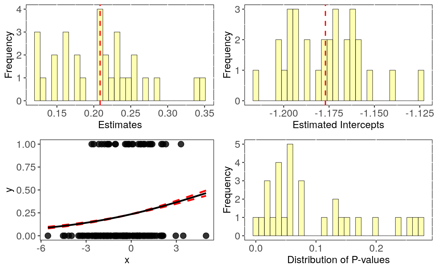
# Simulate Data: set.seed(6987) phy = rtree(150) x = rTrait(n=1,phy=phy) x_sd = rnorm(150,mean = 0.8,sd=0.2) X = cbind(rep(1,150),x) y = rbinTrait(n=1,phy=phy, beta=c(-1,0.5), alpha=.7 ,X=X) dat = data.frame(y, x, x_sd) # Run phylogenetic logistic regression accounting for intraspecific variation: intra_glm <- intra_phyglm(y~x,Vx = "x_sd",data = dat,phy=phy,distrib = "normal")#> Warning: distrib=normal: make sure that standard deviation is provided for Vx#>#> | | | 0% | |== | 3% | |===== | 7% | |======= | 10% | |========= | 13% | |============ | 17% | |============== | 20% | |================ | 23% | |=================== | 27% | |===================== | 30% | |======================= | 33% | |========================== | 37% | |============================ | 40% | |============================== | 43% | |================================= | 47% | |=================================== | 50% | |===================================== | 53% | |======================================== | 57% | |========================================== | 60% | |============================================ | 63% | |=============================================== | 67% | |================================================= | 70% | |=================================================== | 73% | |====================================================== | 77% | |======================================================== | 80% | |========================================================== | 83% | |============================================================= | 87% | |=============================================================== | 90% | |================================================================= | 93% | |==================================================================== | 97% | |======================================================================| 100%#> mean CI_low CI_high #> intercept -1.177 -1.185 -1.169 #> se.intercept 0.246 0.243 0.249 #> pval.intercept 0.000 0.000 0.000 #> estimate 0.208 0.187 0.230 #> se.estimate 0.114 0.112 0.116 #> pval.estimate 0.096 0.065 0.127#> n.intra intercept se.intercept pval.intercept estimate se.estimate #> 1 1 -1.160425 0.2435488 1.891807e-06 0.2104912 0.1114169 #> 2 2 -1.169853 0.2438911 1.613641e-06 0.2081202 0.1101013 #> 3 3 -1.200647 0.2433600 8.071791e-07 0.1428759 0.1049871 #> 4 4 -1.214038 0.2500971 1.208339e-06 0.3386051 0.1187809 #> 5 5 -1.163420 0.2639525 1.044812e-05 0.2868938 0.1195247 #> 6 6 -1.201741 0.2385108 4.691501e-07 0.1239343 0.1118772 #> pval.estimate aic optpar #> 1 0.058862195 153.7267 1.310297 #> 2 0.058723178 153.7237 1.286818 #> 3 0.173548341 155.5238 1.337919 #> 4 0.004362748 148.8378 1.217462 #> 5 0.016382176 150.8696 1.057633 #> 6 0.267961000 156.3245 1.444610