Estimate the influence of clade removal on phylogenetic signal estimates
clade_physig(
  trait.col,
  data,
  phy,
  clade.col,
  n.species = 5,
  n.sim = 100,
  method = "K",
  track = TRUE,
  ...
)
Arguments
| trait.col | The name of a column in the provided data frame with trait to be analyzed (e.g. "Body_mass"). |
|---|---|
| data | Data frame containing species traits with row names matching tips
in |
| phy | A phylogeny (class 'phylo') matching |
| clade.col | The column in the provided data frame which specifies the clades (a character vector with clade names). |
| n.species | Minimum number of species in a clade for the clade to be
included in the leave-one-out deletion analysis. Default is |
| n.sim | Number of simulations for the randomization test. |
| method | Method to compute signal: can be "K" or "lambda". |
| track | Print a report tracking function progress (default = TRUE) |
| ... | Further arguments to be passed to |
Value
The function clade_physig returns a list with the following
components:
trait.col: Column name of the trait analysed
full.data.estimates: Phylogenetic signal estimate (K or lambda)
and the P value (for the full data).
sensi.estimates: A data frame with all simulation
estimates. Each row represents a deleted clade. Columns report the calculated
phylogenetic signal (K or lambda) (estimate), difference between simulation
signal and full data signal (DF), the percentage of change
in signal compared to the full data estimate (perc) and
p-value of the phylogenetic signal with the reduced data (pval).
null.dist: A data frame with estimates for the null distribution
of phylogenetic signal for all clades analysed.
data: Original full dataset.
Details
This function sequentially removes one clade at a time, estimates phylogenetic
signal (K or lambda) using phylosig and stores the
results. The impact of a specific clade on signal estimates is calculated by the
comparison between the full data (with all species) and reduced data estimates
(without the species belonging to a clade).
To account for the influence of the number of species on each clade (clade sample size), this function also estimate a null distribution of signal estimates expected by the removal of the same number of species as in a given clade. This is done by estimating phylogenetic signal without the same number of species in the given clade. The number of simulations to be performed is set by 'n.sim'. To test if the clade influence differs from the null expectation for a clade of that size, a randomization test can be performed using 'summary(x)'.
Output can be visualised using sensi_plot.
Note
The argument "se" from phylosig is not available in this function. Use the
argument "V" instead with intra_physig to indicate the name of the column containing the standard
deviation or the standard error of the trait variable instead.
References
Paterno, G. B., Penone, C. Werner, G. D. A. sensiPhy: An r-package for sensitivity analysis in phylogenetic comparative methods. Methods in Ecology and Evolution 2018, 9(6):1461-1467
Blomberg, S. P., T. Garland Jr., A. R. Ives (2003) Testing for phylogenetic signal in comparative data: Behavioral traits are more labile. Evolution, 57, 717-745.
Pagel, M. (1999) Inferring the historical patterns of biological evolution. Nature, 401, 877-884.
Kamilar, J. M., & Cooper, N. (2013). Phylogenetic signal in primate behaviour, ecology and life history. Philosophical Transactions of the Royal Society B: Biological Sciences, 368: 20120341.
See also
Examples
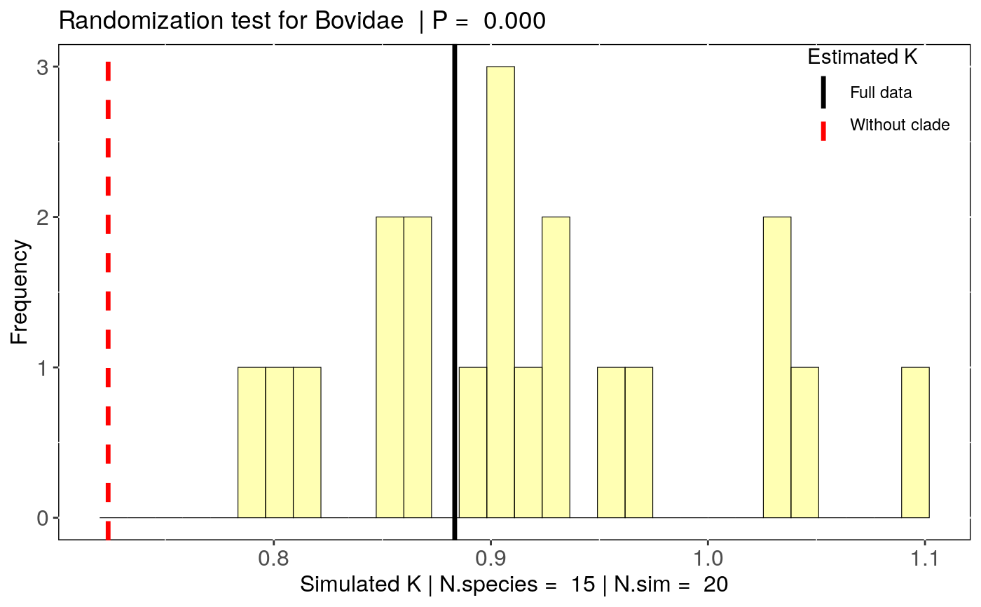
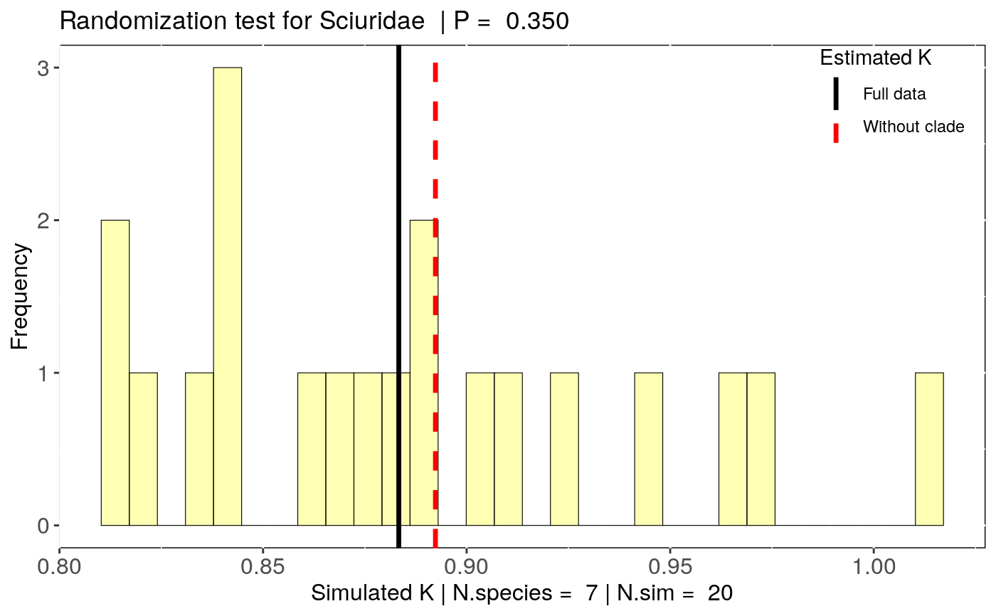
data(alien) alien.data<-alien$data alien.phy<-alien$phy # Logtransform data alien.data$logMass <- log(alien.data$adultMass) # Run sensitivity analysis: clade <- clade_physig(trait.col = "logMass", data = alien.data, n.sim = 20, phy = alien.phy[[1]], clade.col = "family", method = "K")#> Warning: NA's in response or predictor, rows with NA's were removed#> Warning: Some phylo tips do not match species in data (this can be due to NA removal) species were dropped from phylogeny or data#>#> | | | 0% | |= | 1% | |= | 2% | |== | 3% | |=== | 4% | |==== | 5% | |==== | 6% | |===== | 7% | |====== | 8% | |====== | 9% | |======= | 10% | |======== | 11% | |======== | 12% | |========= | 13% | |========== | 14% | |========== | 15% | |=========== | 16% | |============ | 17% | |============= | 18% | |============= | 19% | |============== | 20% | |=============== | 21% | |=============== | 22% | |================ | 23% | |================= | 24% | |================== | 25% | |================== | 26% | |=================== | 27% | |==================== | 28% | |==================== | 29% | |===================== | 30% | |====================== | 31% | |====================== | 32% | |======================= | 33% | |======================== | 34% | |======================== | 35% | |========================= | 36% | |========================== | 37% | |=========================== | 38% | |=========================== | 39% | |============================ | 40% | |============================= | 41% | |============================= | 42% | |============================== | 43% | |=============================== | 44% | |================================ | 45% | |================================ | 46% | |================================= | 47% | |================================== | 48% | |================================== | 49% | |=================================== | 50% | |==================================== | 51% | |==================================== | 52% | |===================================== | 53% | |====================================== | 54% | |====================================== | 55% | |======================================= | 56% | |======================================== | 57% | |========================================= | 58% | |========================================= | 59% | |========================================== | 60% | |=========================================== | 61% | |=========================================== | 62% | |============================================ | 63% | |============================================= | 64% | |============================================== | 65% | |============================================== | 66% | |=============================================== | 67% | |================================================ | 68% | |================================================ | 69% | |================================================= | 70% | |================================================== | 71% | |================================================== | 72% | |=================================================== | 73% | |==================================================== | 74% | |==================================================== | 75% | |===================================================== | 76% | |====================================================== | 77% | |======================================================= | 78% | |======================================================= | 79% | |======================================================== | 80% | |========================================================= | 81% | |========================================================= | 82% | |========================================================== | 83% | |=========================================================== | 84% | |============================================================ | 85% | |============================================================ | 86% | |============================================================= | 87% | |============================================================== | 88% | |============================================================== | 89% | |=============================================================== | 90% | |================================================================ | 91% | |================================================================ | 92% | |================================================================= | 93% | |================================================================== | 94% | |================================================================== | 95% | |=================================================================== | 96% | |==================================================================== | 97% | |===================================================================== | 98% | |===================================================================== | 99% | |======================================================================| 100%summary(clade)#> $`Full data: K phylogenetic signal estimate` #> Trait N.species estimate Pval #> 1 logMass 92 0.8833355 0.001 #> #> $`Summary by clade removal` #> clade.removed N.species estimate DIF.est Change (%) Pval #> 1 Bovidae 15 0.7236622 -0.159673335 18.1 0.001 #> 2 Cervidae 12 0.7700364 -0.113299161 12.8 0.001 #> 3 Macropodidae 8 0.9608746 0.077539057 8.8 0.001 #> 4 Mustelidae 6 0.9348294 0.051493828 5.8 0.001 #> 5 Sciuridae 7 0.8923417 0.009006148 1.0 0.001 #> m.null.estimate Pval.randomization #> 1 0.9179747 0.00 #> 2 0.8977280 0.00 #> 3 0.8917848 0.05 #> 4 0.8877609 0.15 #> 5 0.8857689 0.35 #>#> Warning: Use of `nd$estimate` is discouraged. Use `estimate` instead.#> Warning: Use of `nd$estimate` is discouraged. Use `estimate` instead.